Navigation:  Objects > Loci > Anatomy of a Locus

Recall the definition of a locus: A locus is a set of positions of a driven object as a driver varies over its domain.

Possible driven objects include points, straight objects, circles, arcs, interiors, pictures, function plots, and loci themselves.

Possible drivers are points on paths and parameters.

The domain for a point driver is normally its path, which might be a straight object, a circle, an arc, a polygon or other interior, a function plot, or another point locus. If the point driver is not constructed on a path, you must explicitly select a path to serve as the domain.

The domain for a parameter driver is a numeric domain that you specify when you construct the locus.

Examples of Loci

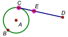
Locus of a point, driven by another point: The illustration below left shows segment CD with end point C attached to circle AB; the illustration below right shows the locus of point E on the segment.

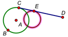
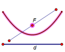
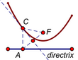
Locus of a point, driven by another point: In the illustration below left, point P is the intersection of line j (the perpendicular bisector of segment CF) and line k (the perpendicular to d through C). This construction guarantees that point P is equally distant from point F and segment d. The illustration below right shows a parabola: the locus of point P as point C moves along segment d.

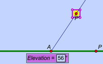
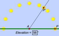
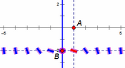
Locus of a picture, driven by a parameter: In the illustration below left, parameter Elevation has been used to rotate point P to P', and a picture has been attached to P'. On the right is the locus of the picture as the parameter varies from 0° to 180°.

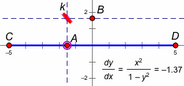
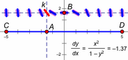
Locus of a segment, driven by a point: In the illustration below left, segment k is constructed to have a slope determined by a calculation involving its x and y values. As driver point A moves along segment CD, the calculation's value changes, and so does the slope of segment k. The locus below right shows the locus of the slope segment for various positions of point A on its domain.

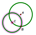
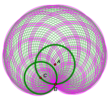
Locus of a circle, driven by a point: In the illustration below left, circle AB was constructed first, and then circle CB was constructed with point C defined on circle AB. Point C is the driver, circle CB is the driven object, and circle AB is the domain. (As before, there’s no need to select the domain, because point C is constructed on it.) The illustration below right shows the resulting locus of circle CB.

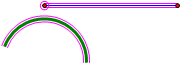
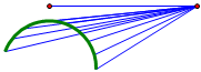
Locus of a segment, driven by an independent point using an arc domain: In the illustrations below, the driver is independent of the domain, so the selections include all three objects: the driver (the left endpoint of the segment), the driven object (the segment), and the domain (the arc). The illustration below right shows the resulting locus of the segment as its endpoint moves along the arc.

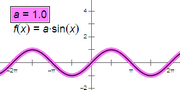
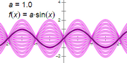
Family of functions (locus of a function plot), driven by a parameter: These illustrations show a family of functions. In this example the driver is parameter a. With the driver and the function plot selected, the command becomes Construct | Family of Functions. The illustration below right shows the resulting family of functions as parameter a varies across its domain. (You can do this same construction using a slider rather than a parameter. When using a slider, the driver would be the adjustable point of the slider.)

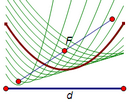
Family of curves (locus of a point locus), driven by another point: These illustrations show a family of point loci. In this example the driver is point F, the focus of the parabola locus. With the driver and the locus selected, the command becomes Construct | Family of Curves. The illustration below right shows the resulting family of parabolas as focus F moves along its segment.

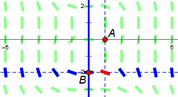
Family of loci (locus of a non-point locus), driven by a point: These illustrations show a family of loci. Driver point B can move along the vertical segment, determining the vertical position of the red slope segment and of the locus of the slope segment. With the driver and the segment locus selected, the command becomes Construct | Family of Loci. The illustration below right shows the resulting family of loci: the slope field of the differential equation used to determine the slope of the red segment.

Two metaphors may help you better understand how the various parts of a locus relate to each other. One way of thinking about a locus with a point driver is as an abstract mathematical function, a function in which the elements of the ordered pairs are not necessarily numbers. For a locus driven by a parameter, the first element of the ordered pair is a specific value of the parameter (a number) and the second element is the corresponding position of the driven geometric object. A locus driven by a point is similar, but the first element is the position of the driver point. Sketchpad moves or varies the independent variable (the driver) along its domain (its path), while keeping track of the position of  the dependent variable (the driven object). Each sample of the locus represents one value of the function, and the entire locus is an approximation of the range of the function. (It’s an approximation because Sketchpad uses only a finite number of ordered pairs — or samples — in constructing the locus.) The abstract mathematical function in this analogy is the construction by which the independent variable (the driver) determines the position of the dependent variable (the driven object).

A second way of thinking about a locus is as a durable form of a traced animation. An animating point or parameter (the driver) moves or varies along its domain and defines the position of some object (the driven object). If you trace that object, you eventually see all of its positions (its locus) for the animated positions or values of the driver.  (Where animation and tracing require time and motion to trace out the locus of an object, a construction of its locus gives you the entire result instantaneously, allowing you to use time and motion to then further explore or manipulate that result.)

Choose Edit | Properties | Plot to set the number of samples and to determine whether the locus is displayed in discrete or continuous form.